library(tidyverse)
# stocks and market index S&P500 from yahoo finance
cme <- read_csv("investment_hw/cme.csv") %>% tibble()
ndaq <- read_csv("investment_hw/ndaq.csv") %>% tibble()
ice <- read_csv("investment_hw/ice.csv") %>% tibble()
spx <- read_csv("investment_hw/spx.csv") %>% tibble()
# risk-free rate is effective-FFR(federal funds rate)
ffr <- read_csv("investment_hw/fedfunds.csv") %>% tibble()
# set period 10years
strt_dd='20140101'; end_dd='20240331'투자분석 과제2
Problems
Answer
(a)
저는 CME group(CME), ICE(ICE), Nasdaq(NDAQ)K 세가지 종목을 선정하였습니다.
선정 배경으로는,
- 제가 거래소 산업에 관심이 많고,
- 세 주식 모두 미국에 상장되어있는 대표적인 글로벌 거래소이며,
- 동일한 거래소 산업이고 S&P500지수의 구성종목이라 동일 선상에서 비교하기 적합할 것으로 보이기 때문입니다.
세 주식의 일별수정주가(Adj. close), 벤치마크지수인 S&P500지수의 일별수정가격, 무위험이자율로 채택한 미연준의 일별 Effective-FFR(Federel Funds Rate)를 활용하였습니다.
기간 : 직전 10년(2014.4 ~ 2024.3)
출처 : [Yahoo Finance](https://finance.yahoo.com/)
산출방법 :
    (월수익률) 지난달 말 대비 월말 수익률
    (월초과수익률) 월수익률 - 월말FFR/12
    (월분산) 월/월초과수익률의 표본표준편차
    (평균수익률) 월/월초과수익률을 산술평균하여 연환산 (x12)
(평균분산) 월분산을 산술평균하여 연환산 (x12)(b)
# tidy data
raw_data <- tibble()
raw_data <- cme %>% mutate(cme=`Adj Close`) %>% select(Date,cme) %>%
  left_join(ndaq %>% mutate(ndaq=`Adj Close`) %>% select(Date,ndaq)) %>%
  left_join(ice %>% mutate(ice=`Adj Close`) %>% select(Date,ice)) %>%
  left_join(spx %>% mutate(spx=`Adj Close`) %>% select(Date,spx)) %>%
  mutate(day=gsub("-","",Date)) %>%
  mutate(year=substr(day,1,4)) %>%
  mutate(month=substr(day,1,6)) %>%
  filter(day>=strt_dd,day<=end_dd) %>%
  left_join(ffr %>%
              mutate(ffr=FEDFUNDS/100,
                     month=substr(gsub("-","",as.character(DATE)),1,6)) %>%
              select(month,ffr)) %>%
  select(year,month,day,cme,ndaq,ice,spx,ffr,Date)
# using monthly return
monthly_raw <- tibble()
monthly_raw <- raw_data %>%
  group_by(year,month) %>%
  arrange(day %>% desc()) %>%
  slice(1) %>%
  pivot_longer(.,c("cme","ndaq","ice","spx"),
               names_to = "name",values_to = "price") %>%
  ungroup() %>%
  arrange(name,year,month) %>%
  mutate(return=price/lag(price)-1) %>%  # monthly return
  mutate(excess_return=return-ffr*(1/12)) %>%
  filter(as.integer(month)>=201404)

# calculate arithmatic mean&var and var-cov matrix of excess return of stocks
monthly_stat <- tibble()
monthly_stat <- monthly_raw %>%
  ungroup() %>%
  group_by(name) %>%
  summarise(avg_excess=mean(excess_return)*12,
            var_excess=sd(excess_return)^2*12,
            avg_return=mean(return)*12,
            var_return=sd(return)^2*12,
            avg_rf=mean(ffr)) # Annualized
# Cov matrix
variance_matrix <- monthly_raw %>%
  ungroup() %>%
  select(month,name,excess_return) %>%
  pivot_wider(names_from = "name", values_from = "excess_return") %>%
  select(cme,ice,ndaq,spx) %>%
  var()
# Corr matrix
cor_matrix <- monthly_raw %>%
  ungroup() %>%
  select(month,name,excess_return) %>%
  pivot_wider(names_from = "name", values_from = "excess_return") %>%
  select(cme,ice,ndaq,spx) %>%
  cor()
위 방법을 기준으로 산출한 각 주식의 평균초과수익률(연환산) 및 공분산행렬은 아래와 같습니다.
Excess return : CME 15.0%, ICE 14.4%, Nasdaq 18.8%
monthly_stat# A tibble: 4 × 6
name avg_excess var_excess avg_return var_return avg_rf
<chr> <dbl> <dbl> <dbl> <dbl> <dbl>
1 cme 0.150 0.0340 0.165 0.0340 0.0141
2 ice 0.144 0.0414 0.158 0.0415 0.0141
3 ndaq 0.188 0.0415 0.202 0.0413 0.0141
4 spx 0.101 0.0229 0.115 0.0229 0.0141Variance-Covariance Matrix of three stocks&Benchmark index
variance_matrix cme ice ndaq spx
cme 0.0028310476 0.001767299 0.001138796 0.0008194417
ice 0.0017672988 0.003452184 0.002149990 0.0016652315
ndaq 0.0011387956 0.002149990 0.003456322 0.0016308630
spx 0.0008194417 0.001665231 0.001630863 0.0019071007Correlation Matrix of three stocks&Benchmark index
cor_matrix cme ice ndaq spx
cme 1.0000000 0.5653136 0.3640534 0.3526612
ice 0.5653136 1.0000000 0.6224185 0.6489942
ndaq 0.3640534 0.6224185 1.0000000 0.6352191
spx 0.3526612 0.6489942 0.6352191 1.0000000(c)
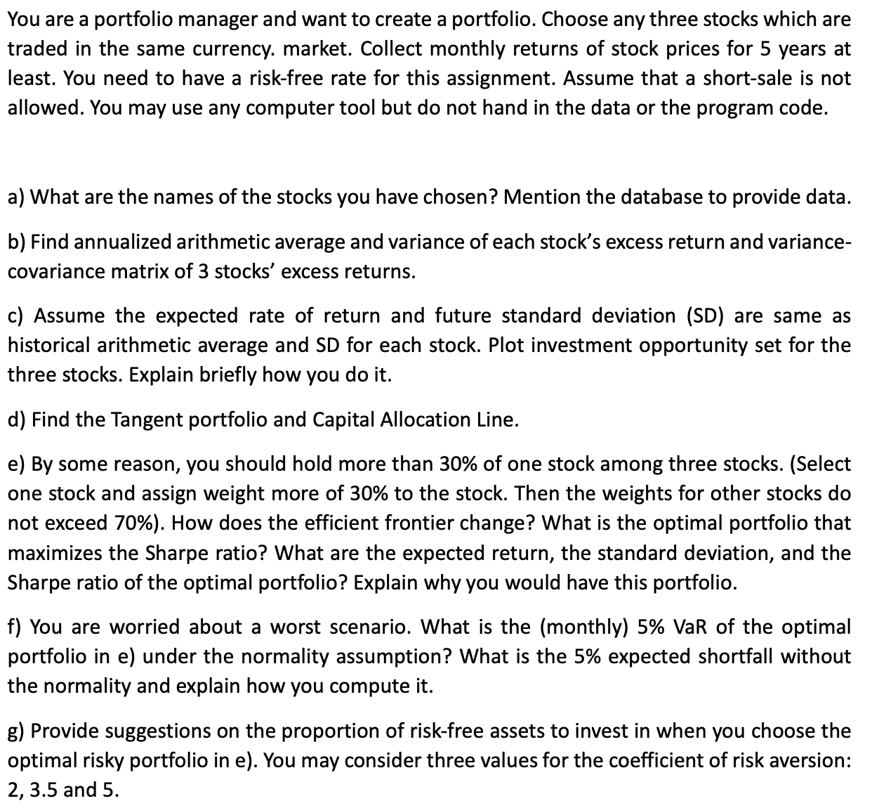
각 주식의 기대수익률과 미래변동성이 과거실현값과 동일하다고 가정하겠습니다.
공매도는 없다고 가정하였으므로 각 주식의 비중이 양수가 되도록 설정하고, 먼저 두개의 주식으로 구성된 포트폴리오의 efficient frontier를 각각 구하도록 하겠습니다.
그 다음, 하나의 주식과 다른 두 주식의 포트폴리오를 재결합하면 새로운 포트폴리오를 구성할 수 있으며, 이를 반복하여 efficient frontier를 도식화할 수 있습니다.
아래 코드에서는 ICE의 구성비중을 5%, 10%, … , 95%로 고정하고 CME-Nasdaq 포트폴리오와 재결합을 반복하여 efficient frontier를 구현하였습니다.
# Portfolio return/vol of variance combinations three stocks
portfolio <- tibble()
portfolio <- tibble(cme=seq(0,1,0.002),ice=seq(1,0,-0.002)) %>%
  union_all(.,tibble(cme=seq(0,1,0.002),ice=0)) %>%
  union_all(.,tibble(cme=0,ice=seq(1,0,-0.002)))

for(i in seq(0.05,0.95,0.05)){portfolio <- portfolio %>%
  union_all(.,tibble(cme=seq(0,1-i,0.005),ice=i))}
for(i in seq(0.25,0.30,0.01)){portfolio <- portfolio %>%
  union_all(.,tibble(cme=seq(0,1-i,0.005),ice=i))}

portfolio <- portfolio %>%
  mutate(ndaq=1-cme-ice) %>%
  mutate(return=cme*monthly_stat$avg_return[1]
         +ice*monthly_stat$avg_return[2]
         +ndaq*monthly_stat$avg_return[3],
         vol=sqrt(cme^2*monthly_stat$var_return[1]
                  +ice^2*monthly_stat$var_return[2]
                  +ndaq^2*monthly_stat$var_return[3]
                  +2*cme*ice*variance_matrix[2]
                  +2*cme*ndaq*variance_matrix[3]
                  +2*ndaq*ice*variance_matrix[7])) %>%
  mutate(sharpe=(return-monthly_stat$avg_rf[1])/vol)

plot_portfolio <- ggplot(data=portfolio,mapping=aes(x=vol,y=return))+
  geom_point(data=portfolio %>% filter(ndaq==0),size=0.5,color="red")+
  geom_point(data=portfolio %>% filter(ice==0),size=0.5,color="blue")+
  geom_point(data=portfolio %>% filter(cme==0),size=0.5,color="green")+
  scale_x_continuous(limits=c(0.08,0.22))+
  scale_y_continuous(limits=c(0.15,0.21))+
  labs(title = "Invest Opportunity of three stocks",
       x="standard deviation",y="expected return") +
  annotate(geom="text",x=0.182,y=0.17,label="CME")+
  annotate(geom="text",x=0.202,y=0.205,label="Nasdaq")+
  annotate(geom="text",x=0.202,y=0.162,label="ICE")+
  theme_bw()

plot_combination <- plot_portfolio +
  geom_point(data=portfolio %>% filter(cme!=0&ice!=0&ndaq!=0),size=1,
  color="black",alpha=0.1)

plot_combination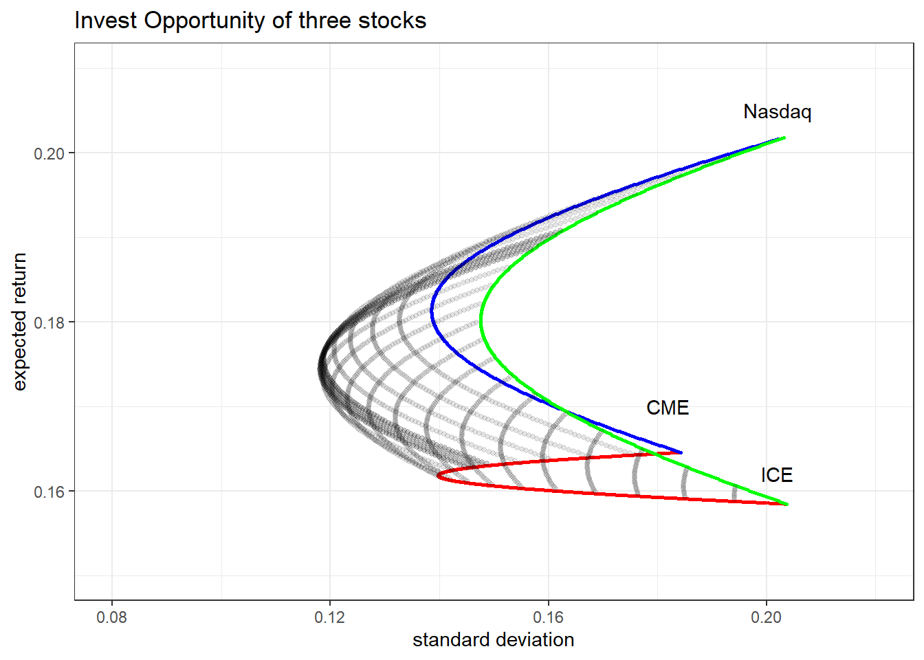
(d)
Tangent p/f는 Sharpe r/o를 최대화시키는 세 주식의 조합으로, 위에서 도식화한 투자기회에 대하여 무위험이자율을 y절편으로 가지는 접선을 그려서 시각화할 수 있습니다.
접선의 기울기는 포트폴리오의 초과수익률을 변동성으로 나눈 값으로 Sharpe r/o가 되므로, 이 접선이 CAL에 해당합니다.
sharpe=max(portfolio$sharpe)
tangent <- tibble(vol=seq(0.08,0.17,0.01)) %>%
  mutate(return=monthly_stat$avg_rf[1]+sharpe*vol)

plot_tangent <- plot_combination+
  geom_line(data=tangent)+
  scale_x_continuous(limits=c(0.04,0.26))+
  scale_y_continuous(limits=c(0.11,0.25))+
  annotate(geom="text",x=0.125,y=0.23,label="CAL, y=1.3667x+0.0141")+
  annotate(geom="text",x=0.125,y=0.22,label="sharpe r/o=1.3667")+
  annotate(geom="text",x=0.1,y=0.18,label="Tangent p/f")
Scale for x is already present.
Adding another scale for x, which will replace the existing scale.
Scale for y is already present.
Adding another scale for y, which will replace the existing scale.plot_tangent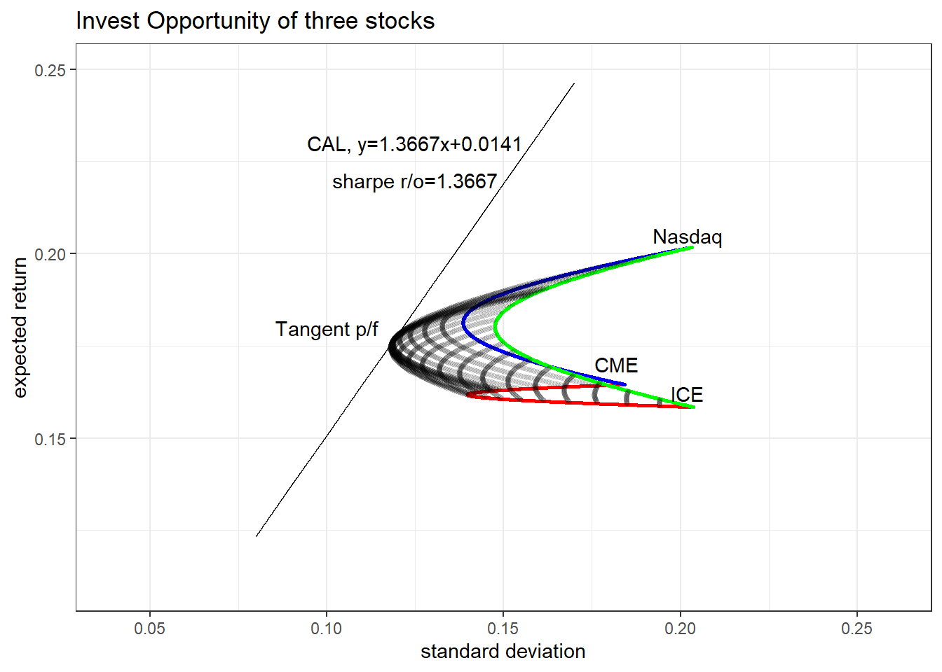
이 때, Tangent p/f의 기대수익률/변동성/구성비율은 아래와 같습니다.
portfolio %>% arrange(sharpe %>% desc()) %>% slice(1)# A tibble: 1 × 6
cme ice ndaq return vol sharpe
<dbl> <dbl> <dbl> <dbl> <dbl> <dbl>
1 0.36 0.27 0.37 0.177 0.119 1.37(e)
Tangent p/f에서 CME, Nasdaq의 비중은 각각 36%, 37%로 이미 30%를 초과하였습니다. 따라서 30%를 초과보유할 주식을 선정할 때 두 주식을 선정한다면 최적포트폴리오는 (d)의 Tangent p/f와 동일할 것 입니다.
한편, ICE를 선정한다면 (d)의 Tangent p/f 구성이 불가능합니다. 이 경우 새로운 efficient frontier는 아래와 같이 도식화할 수 있으며, 새로운 최적포트폴리오는 ICE의 비중이 정확히 30%일 때 결정됩니다.
# Set ice>=0.3
portfolio2 <- portfolio %>% filter(ice>=0.3)
sharpe2=max(portfolio2$sharpe)
tangent2 <- tibble(vol=seq(0.1,0.14,0.01)) %>%
  mutate(return=monthly_stat$avg_rf[1]+sharpe2*vol)

portfolio2 %>% arrange(desc(sharpe))
# A tibble: 1,905 × 6
cme ice ndaq return vol sharpe
<dbl> <dbl> <dbl> <dbl> <dbl> <dbl>
1 0.34 0.3 0.36 0.176 0.119 1.36
2 0.34 0.3 0.36 0.176 0.119 1.36
3 0.345 0.3 0.355 0.176 0.119 1.36
4 0.345 0.3 0.355 0.176 0.119 1.36
5 0.335 0.3 0.365 0.176 0.119 1.36
6 0.335 0.3 0.365 0.176 0.119 1.36
7 0.35 0.3 0.35 0.176 0.119 1.36
8 0.35 0.3 0.35 0.176 0.119 1.36
9 0.33 0.3 0.37 0.176 0.119 1.36
10 0.33 0.3 0.37 0.176 0.119 1.36
# ℹ 1,895 more rowsplot_tangent2 <- plot_portfolio +
geom_point(data=portfolio2 %>% filter(cme!=0&ice!=0&ndaq!=0),
size=1,color="black",alpha=0.2)+
geom_line(data=tangent2)+
annotate(geom="text",x=0.117,y=0.2,label="CAL, y=1.3639x+0.0141")+
annotate(geom="text",x=0.117,y=0.193,label="sharpe r/o=1.3639")+
annotate(geom="text",x=0.11,y=0.18,label="Optimal p/f")
plot_tangent2
Optimal p/f의 기대수익률/변동성/구성비율은 아래와 같습니다.
optimal <- portfolio2 %>% arrange(sharpe %>% desc()) %>% slice(1)
optimal
# A tibble: 1 × 6
cme ice ndaq return vol sharpe
<dbl> <dbl> <dbl> <dbl> <dbl> <dbl>
1 0.34 0.3 0.36 0.176 0.119 1.36(f)
먼저, 포트폴리오의 연환산수익률이 정규분포를 따른다면 표준정규분포표를 참조하여 Value at Risk를 다음과 같이 산출할 수 있습니다.
\[5\%\;VaR=E(r_p)-1.65\sigma_p=0.176-1.65\times 0.119=-1.99\%\]
VaR=optimal$return-1.65*optimal$vol; VaR[1] -0.01990571만약 수익률의 분포가 정규분포가 아니라면, Historical VaR 및 ES(Expected Shortfall)을 산출할 수 있습니다. 이를 데이터의 참조기간인 과거 10년간 최적포트폴리오의 월수익률이 필요합니다.
위의 최적포트폴리오는 CME 34%, ICE 30%, Nasdaq 36%로 구성된 포트폴리오이므로, 거래비용 등을 무시하고 매월말 포트폴리오의 구성비율을 조정한다고 가정하고 포트폴리오의 명목금액을 \(P_t\), 각 주식의 \((t,t+1)\) 월수익률을 \(r_{t,k}\)라고 한다면 \((t,t+1)\)간 포트폴리오의 월수익률 \(r_t\)는 다음과 같습니다.
\[P_{t+1}=0.34\times P_t\times (1+r_{t,cme})+0.3\times P_t\times (1+r_{t,ice})+0.36\times P_t\times (1+r_{t,ndaq})\]
\[\Rightarrow 1+r_t=\frac{P_{t+1}}{P_t}=0.34\times (1+r_{t,cme})+0.3\times (1+r_{t,ice})+0.36\times (1+r_{t,ndaq})\]
이를 적용하면 과거 10년간 최적포트폴리오의 월수익률 120개를 얻을 수 있습니다.
이를 오름차순으로 정렬하면 Historical 5% VaR은 6번째 관측값이며, 5% ES는 6개의 관측값의 평균으로 산출할 수 있습니다. 이는 월수익률 기반 VaR 및 ES이므로 \(\sqrt{12}\)를 곱하여 연환산하도록 하겠습니다.
optimal_monthly <- tibble()
optimal_monthly <- monthly_raw %>%
  select(month,name,return) %>%
  pivot_wider(names_from = "name", values_from = "return") %>%
  mutate(pf_return=optimal$cme*(1+cme)+optimal$ice*(1+ice)+optimal$ndaq*(1+ndaq)-1) %>%
  select(month,cme,ice,ndaq,pf_return) %>%
  arrange(pf_return) %>%
  slice(1:6)
optimal_monthly
# A tibble: 6 × 5
month cme ice ndaq pf_return
<chr> <dbl> <dbl> <dbl> <dbl>
1 202204 -0.0779 -0.123 -0.117 -0.106
2 202002 -0.0842 -0.105 -0.119 -0.103
3 202003 -0.127 -0.0917 -0.0697 -0.0957
4 202209 -0.0899 -0.101 -0.0448 -0.0769
5 202201 0.00455 -0.0739 -0.147 -0.0734
6 202205 -0.0935 -0.116 -0.0134 -0.0714Annualized 5% VaR은 -24.78%, ES는 -30.38%입니다.
정규분포 가정 하에 산출한 VaR과 큰 차이가 나는 이유는 지난 22년 Covid-19 팬데믹으로 인해 이례적으로 주가가 월 7% 이상 하락하는 급락장이 지속(Left fat tail)되었는데, 이때의 outlier 표본이 Historical VaR 산출을 지배한 반면 정규분포 근사시에는 반영되지 않아 차이가 발생하는 것으로 추정됩니다.
hist_VaR <- optimal_monthly$pf_return[6]*sqrt(12)
hist_ES <- mean(optimal_monthly$pf_return[1:6])*sqrt(12)
paste(round(hist_VaR,6), round(hist_ES,6) , round(VaR,6), sep=" / ")
[1] "-0.247279 / -0.303873 / -0.019906"(g)
위의 최적포트폴리오와 무위험자산을 이용하여 투자를 결정한다면, 최종적인 포트폴리오의 기대수익률 및 변동성은 자본배분선(\(E(r_p)=1.3639\sigma_p+0.0141\)) 위에서 결정될 것입니다.
이때, 무위험자산의 비중은 투자자의 위험회피정도에 따른 효용함수 \(U=E(r_p)-\frac{1}{2}A\sigma_p^2\)를 최대화시키는 수준에서 결정됩니다.
이에 따라 산출한 무위험자산의 비중은 모든 경우(A=2, 3.5, 5)에서 0이 됩니다. 이는 과거기간 중 제로금리 기간이 다소 길어 무위험자산의 수익률이 낮은 반면, 선정한 주식의 기대수익률은 상대적으로 높아 일어난 것으로 추정됩니다.
부가적으로, 무위험자산의 비중 산식 \(r^*=1-\frac{E(r_p)-r_f}{A\sigma_p^2}\)를 역산하여 위험회피정도 \(A\)를 역산해보면, 약 11.48까지는 최적포트폴리오를 100% 보유하는 것이 효용을 극대화시키는 투자결정입니다.
# Utility function to verify risk-free asset ratio
utility <- tibble(vol=seq(optimal$vol,0,-0.0001)) %>%
  mutate(return=sharpe2*vol+monthly_stat$avg_rf[1]) %>%
  mutate(rf_ratio=(optimal$return-return)/(optimal$return-monthly_stat$avg_rf[1])) %>%
  mutate(a2=return-0.5*2*vol^2,
         a3.5=return-0.5*3.5*vol^2,
         a5=return-0.5*5*vol^2)
utility %>% arrange(desc(a5)) %>% slice(1)
# A tibble: 1 × 6
vol return rf_ratio a2 a3.5 a5
<dbl> <dbl> <dbl> <dbl> <dbl> <dbl>
1 0.119 0.176 0 0.162 0.151 0.141(optimal$return-monthly_stat$avg_rf[1])/optimal$vol^2[1] 11.48027