library(tidyverse)
birds_caribbean <- tibble("dates"=c(0.00,0.00,0.04,0.21,0.29,
0.54,0.63,0.88,0.96,1.25,
1.67,1.75,1.84,1.96,2.01,
2.51,2.72,3.30,3.51,4.05,
4.85,6.94,8.73,10.57,11.11,
12.45,14.00,17.30,17.92,18.05,
18.43,22.48,22.48,23.48,26.32,
26.45,28.87))경영통계분석 과제1
1. Type of variables
Question
Identify whether the following variables are numerical or categorical. If numerical, state whether the variable is discrete or continuous. If categorical, state whether the variable is nominal or ordinal.
a. Number of companies going bankrupt in a year.
: Numerical and Discrete
b. Petal area of rose flowers.
: Numerical and Continuous
c. Key on the musical scale.
: Categorical and Ordinal
d. Heart beats per minute of a Tour de France cyclist, averaged over the duration of the race.
: Numerical and Continuous
e. Stage of fruit ripeness.
: Categorical and Ordinal
f. Angle of flower orientation relative to position of the sun.
: Numerical and Continuous
g. Tree species
: Categorical and Nominal
h. year of birth
: Numerical and Discrete
i. Gender
: Categorical and Nominal
j. Birth weight
: Numerical and Continuous
2. Discrete data
Question
Birds of the Caribbean islands of the Lesser Antilles are descended from immigrants originating from larger islands and the nearby mainland. The data presented here are the approximate dates of immigration, in millions of years, of each of 37 bird species now present on the Lesser Antilles. The dates were calculated from the difference in mitochondrial DNA sequences between each of the species and its closest living relative on larger islands or the mainland.
birds_caribbean$dates [1] 0.00 0.00 0.04 0.21 0.29 0.54 0.63 0.88 0.96 1.25 1.67 1.75
[13] 1.84 1.96 2.01 2.51 2.72 3.30 3.51 4.05 4.85 6.94 8.73 10.57
[25] 11.11 12.45 14.00 17.30 17.92 18.05 18.43 22.48 22.48 23.48 26.32 26.45
[37] 28.87a. Plot the data in a histogram and describe the shape of the frequency distribution.
ggplot(data=birds_caribbean, aes(x=dates))+
  geom_histogram(binwidth=5, boundary=0, color="black",fill="darkred")+
  scale_x_continuous(breaks = seq(0,30,5)) +
  theme_bw()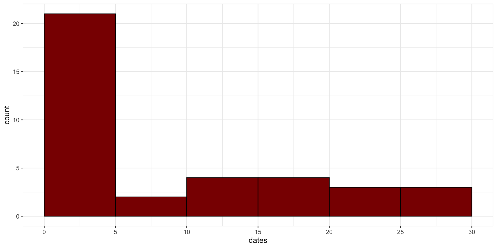
히스토그램은 위와 같으며, 0~5구간에 전체 37종의 조류 중 20종 이상이 넘는 빈도가 집중되어 있습니다. 이는 과반 이상의 조류가 비교적 최근인 500만년 이내에 Lesser Antilles섬으로 이주해왔다는 것을 의미합니다. 나머지 약 15종의 조류는 각각 2~4종씩 ~1천만년, ~1500만년, … , ~3천만년 구간에 고르게 분포되어 있습니다.
b. By viewing the graph alone, approximate the mean and median of the distribution. Which should be greater? Explain your reasoning.
: 히스토그램은 왼쪽으로 치우쳐져 있으며, 이는 \(Skewness>>0\)이라는 것을 말합니다. 이러한 경우 평균은 중간값보다 크게 형성되고, 오른쪽 꼬리가 다소 긴 점을 감안하여 추정해보면, 중간값은 약 4, 평균은 약 10일 것으로 보입니다.
c. Calculate the mean and median. Was your intuition in part (b) correct?
birds_caribbean %>%
  summarise(mean=mean(dates),
            mid=median(dates))
# A tibble: 1 × 2
mean mid
<dbl> <dbl>
1 8.66 3.51: 대략적인 경향성은 맞습니다. 실제 중간값은 3.51 및 평균은 8.66입니다.
d. Calculate the first and third quantiles and the inter quartile range.
birds_caribbean %>%
  reframe(quantile=quantile(dates))
# A tibble: 5 × 1
quantile
<dbl>
1 0
2 1.25
3 3.51
4 17.3
5 28.9 : First(25%) quantiles은 1.25이며, third(75%) quantiles은 17.30입니다. IQR은 16.05입니다.
e. Draw a box plot for these data
ggplot(birds_caribbean, aes(x=dates))+
  geom_boxplot()+
  scale_y_continuous(limits=c(-0.5,0.5))+
  theme_bw()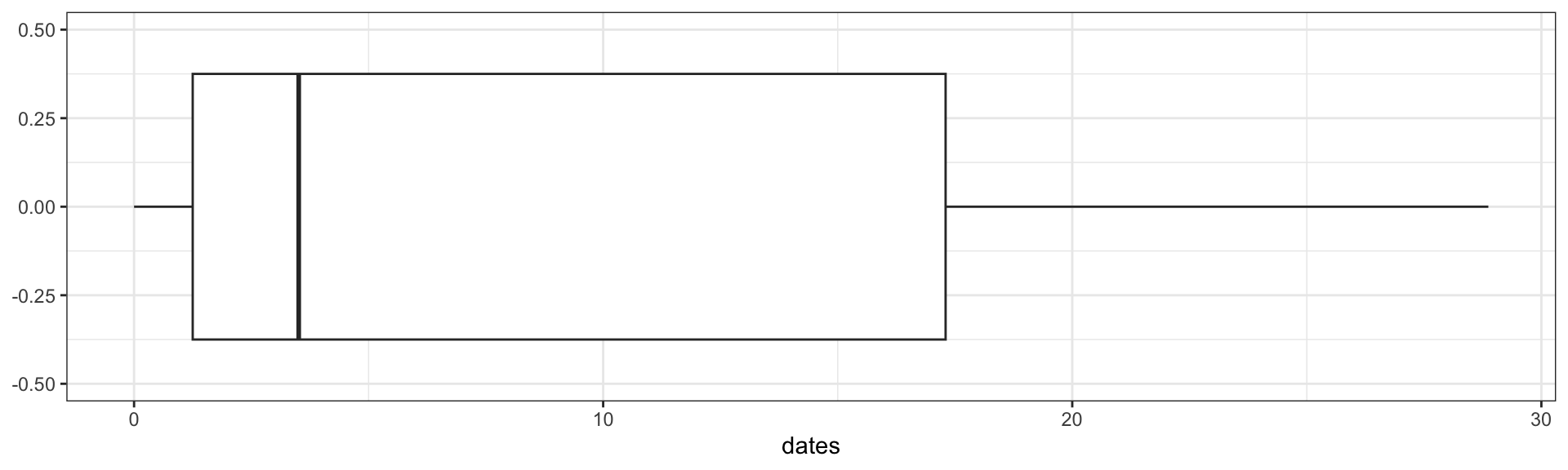
3. Histogram
Question
Francis Galton presented the following data on the flight speeds of 3207 “old” homing pigeons traveling at least 90 miles.
a. What type of graph is this?
: Histogram
b. Examine the graph and visually determine the approximate value of the mean (to the nearest 100 yards per minute). Explain how you obtained your estimate.
: 그래프는 bell-shape의 히스토그램이며, 오른쪽 꼬리가 긴 형태입니다. 아마 \(skewness>0\)일 것으로 보이며, 평균은 중간값보다 클 것 입니다.
그래프에서 중간값은 오른쪽 꼬리가 긴 분포를 고려할 때 약 1,000일 것으로 추정할 수 있는데, 평균값은 이보다 큰 약 1,100이 될 것으로 추정됩니다.
c. Examine the graph and visually determine the approximate value of the median (to the nearest 100 yards per minute). Explain how you obtain your estimate.
: 그래프에서 900~1000이 중심막대인데, bell-shape와 오른쪽 꼬리가 긴 분포를 고려할 때, 중간값은 약 1,000이 될 것으로 추정됩니다.
d. Examine the graph and visually determine the approximate value of the mode (to the nearest 100 yards per minute). Explain how you obtained your estimate.
: 최빈값은 가장 많은 빈도를 가지는 값 또는 구간으로, 히스토그램의 가장 높은 막대인 1000~1100에 존재할 것입니다. 막대 왼쪽에 빈도가 더 많은 점을 고려할 때 최빈값은 약 1,000일 것으로 보입니다.
e. Examine the graph and visually determine the approximate value of the standard deviation (to the nearest 100 yards per minute). Explain how you obtained your estimate.
: 먼저, 정규분포를 따르는 확률변수에 대해 다음 식이 성립합니다.
\[for\;X\;\sim\;Normal\;Dist.\;then\;P[-\sigma<X<\sigma]\approx 68.2\%\]
문제의 히스토그램은 bell-shape로 정규분포를 따른다고 가정하는 것에 큰 문제는 없어보입니다. 히스토그램에서 어림잡아봤을 때, 약 \(1,100\pm 200\) 구간이 70~80%에 해당한다고 보여지는데, (\(P[900<x<1300]=70\sim80\%\))
이는 (b)의 추정 평균을 이용하면 \(평균\pm 200\)입니다. 즉, 히스토그램이 정규분포를 따른다고 가정하면, 히스토그램의 형태는 \(N(1050,\sigma^2=(200-\alpha)^2)\)의 확률밀도함수가 유사할 것입니다. 한편, 히스토그램은 오른쪽 꼬리가 긴 형태를 가지고 있어 변동성은 정규분포 대비 다소 클 것입니다.
따라서, 최종적으로 히스토그램 데이터의 표준편차는 약 200으로 추정됩니다.
4. Sample Statistics
handheight <- tibble("person"=c("A","B","C","D","E"),
                     "hand"=c(17,15,19,17,21),
                     "height"=c(150,154,169,172,175))
handheight
# A tibble: 5 × 3
person hand height
<chr> <dbl> <dbl>
1 A 17 150
2 B 15 154
3 C 19 169
4 D 17 172
5 E 21 175a. Calculate the sample variances for hand and height, respectively.
표분 분산은 \(s_x^2=\frac{\sum_{k=1}^n(X_k-\bar{X})^2}{n-1}\)입니다.
sample_var <- handheight %>%
  mutate(hand_tmp=hand-mean(handheight$hand),
         height_tmp=height-mean(handheight$height)) %>%
  mutate(hand_tmp=hand_tmp^2,
         height_tmp=height_tmp^2) %>%
  summarise(s_var_hand=sum(hand_tmp)/4,
            s_var_height=sum(height_tmp)/4)
sample_var
# A tibble: 1 × 2
s_var_hand s_var_height
<dbl> <dbl>
1 5.2 126.b. Calculate the sample covariance.
표본 공분산은 \(s_{xy}=\frac{\sum_{k=1}^n(X_k-\bar{X})(Y_k-\bar{Y})}{n-1}\) 입니다.
sample_cov <- handheight %>%
  mutate(s_cov_tmp=(hand-mean(handheight$hand))*(height-mean(handheight$height))) %>%
  summarise(s_cov=sum(s_cov_tmp)/4)
sample_cov
# A tibble: 1 × 1
s_cov
<dbl>
1 18.5c. Calculate the sample correlation and interpret the result.
표본 상관계수는 \(r_{xy}=\frac{s_{x,y}}{s_xs_y}\) 입니다.
sample_corr=sample_cov$s_cov/sqrt(sample_var$s_var_hand*sample_var$s_var_height)
sample_corr
[1] 0.7213147표본상관계수는 약 0.72이며, 이는 두 변수간에 강한 양의 선형관계가 존재하는 것을 말합니다. 즉, 손의 크기와 키 사이에는 양의 상관관계가 있어 손이 큰 집단은 키도 큰 경향이 있고, 키가 큰 집단은 손도 큰 경향이 있다는 것을 의미합니다.
R 내장함수
참고로, R 내장함수는 표본연산을 기본으로 하고 있어 내장함수를 이용하여 표현 가능합니다.
var(handheight$hand)[1] 5.2var(handheight$height)[1] 126.5cov(handheight$hand,handheight$height)[1] 18.5cor(handheight$hand,handheight$height)[1] 0.7213147