1  빅데이터와 금융자료 분석 CH1

import numpy as np
import pandas as pd

missdict = {'f1': [1, 2, 3, 4, 5, 6, 7, 8, 9, 10],
            'f2': [10., None, 20., 30., None, 50., 60., 70., 80., 90.],
            'f3': ['A', 'A', 'A', 'A', 'B', 'B', 'B', 'B', 'C', 'C']}
missdata = pd.DataFrame( missdict )
missdata.info()

<class 'pandas.core.frame.DataFrame'>
RangeIndex: 10 entries, 0 to 9
Data columns (total 3 columns):
 #   Column  Non-Null Count  Dtype  
---  ------  --------------  -----  
 0   f1      10 non-null     int64  
 1   f2      8 non-null      float64
 2   f3      10 non-null     object 
dtypes: float64(1), int64(1), object(1)
memory usage: 368.0+ bytes

missdata.isna().mean()

f1    0.0
f2    0.2
f3    0.0
dtype: float64

tmpdata1 = missdata.dropna()
tmpdata1

	f1	f2	f3
0	1	10.0	A
2	3	20.0	A
3	4	30.0	A
5	6	50.0	B
6	7	60.0	B
7	8	70.0	B
8	9	80.0	C
9	10	90.0	C

tmpdata2 = missdata.dropna( subset=['f3'] )
tmpdata2

	f1	f2	f3
0	1	10.0	A
1	2	NaN	A
2	3	20.0	A
3	4	30.0	A
4	5	NaN	B
5	6	50.0	B
6	7	60.0	B
7	8	70.0	B
8	9	80.0	C
9	10	90.0	C

numdata = missdata.select_dtypes(include=['int64', 'float64'])
tmpdata3 = numdata.fillna( -999, inplace=False )
tmpdata3.describe()

	f1	f2
count	10.00000	10.000000
mean	5.50000	-158.800000
std	3.02765	443.562297
min	1.00000	-999.000000
25%	3.25000	12.500000
50%	5.50000	40.000000
75%	7.75000	67.500000
max	10.00000	90.000000

numdata.mean()

f1     5.50
f2    51.25
dtype: float64

tmpdata4 = numdata.fillna( numdata.mean(), inplace=False )
tmpdata4

	f1	f2
0	1	10.00
1	2	51.25
2	3	20.00
3	4	30.00
4	5	51.25
5	6	50.00
6	7	60.00
7	8	70.00
8	9	80.00
9	10	90.00

missdata.groupby('f3')['f2'].mean()

f3
A    20.0
B    60.0
C    85.0
Name: f2, dtype: float64

missdata.groupby('f3')['f2'].transform('mean')

0    20.0
1    20.0
2    20.0
3    20.0
4    60.0
5    60.0
6    60.0
7    60.0
8    85.0
9    85.0
Name: f2, dtype: float64

tmpdata5 = numdata.copy()
tmpdata5['f2'].fillna( missdata.groupby('f3')['f2'].transform('mean'), inplace=True)
tmpdata5

/var/folders/n2/jbh_0_091bx8qgz7j87t2qwc0000gp/T/ipykernel_25894/622840210.py:2: FutureWarning: A value is trying to be set on a copy of a DataFrame or Series through chained assignment using an inplace method.
The behavior will change in pandas 3.0. This inplace method will never work because the intermediate object on which we are setting values always behaves as a copy.

For example, when doing 'df[col].method(value, inplace=True)', try using 'df.method({col: value}, inplace=True)' or df[col] = df[col].method(value) instead, to perform the operation inplace on the original object.


  tmpdata5['f2'].fillna( missdata.groupby('f3')['f2'].transform('mean'),inplace=True)

	f1	f2
0	1	10.0
1	2	20.0
2	3	20.0
3	4	30.0
4	5	60.0
5	6	50.0
6	7	60.0
7	8	70.0
8	9	80.0
9	10	90.0

missdata_tr = missdata.dropna()
x_tr = missdata_tr[['f1']]
y_tr = missdata_tr['f2']

from sklearn.linear_model import LinearRegression
model = LinearRegression()
model.fit( x_tr, y_tr )

missdata_ts = missdata [ missdata.isnull().any(axis=1) ]
x_ts = missdata_ts[['f1']]

predicted_values = model.predict( x_ts )
tmpdata6 = missdata.copy()
tmpdata6.loc[ tmpdata6['f2'].isnull(), 'f2'] = predicted_values
tmpdata6

	f1	f2	f3
0	1	10.000000	A
1	2	14.191176	A
2	3	20.000000	A
3	4	30.000000	A
4	5	41.985294	B
5	6	50.000000	B
6	7	60.000000	B
7	8	70.000000	B
8	9	80.000000	C
9	10	90.000000	C

missdata_num = missdata.copy()
missdata_num['f3']=missdata_num['f3'].map({'A':1,'B':2,'C':3})

missdata_num

	f1	f2	f3
0	1	10.0	1
1	2	NaN	1
2	3	20.0	1
3	4	30.0	1
4	5	NaN	2
5	6	50.0	2
6	7	60.0	2
7	8	70.0	2
8	9	80.0	3
9	10	90.0	3

from sklearn.impute import KNNImputer
imputer = KNNImputer(n_neighbors=2)
tmpdata7 = imputer.fit_transform(missdata_num)

pd.DataFrame( tmpdata7 )

	0	1	2
0	1.0	10.0	1.0
1	2.0	15.0	1.0
2	3.0	20.0	1.0
3	4.0	30.0	1.0
4	5.0	40.0	2.0
5	6.0	50.0	2.0
6	7.0	60.0	2.0
7	8.0	70.0	2.0
8	9.0	80.0	3.0
9	10.0	90.0	3.0

outdict = {'A': [10, 0.02, 0.3, 40, 50, 60, 712, 80, 90, 1003],
           'B': [0.05, 0.00015, 25, 35, 45, 205, 65, 75, 85, 3905]}
outdata = pd.DataFrame( outdict )

Q1 = outdata.quantile(0.25)
Q3 = outdata.quantile(0.75)
IQR = Q3 - Q1
lower_bound = Q1 - 1.5 * IQR
upper_bound = Q3 + 1.5 * IQR

((outdata < lower_bound) | (outdata > upper_bound))

	A	B
0	False	False
1	False	False
2	False	False
3	False	False
4	False	False
5	False	True
6	True	False
7	False	False
8	False	False
9	True	True

outliers = ((outdata < lower_bound) | (outdata > upper_bound)).any(axis=1)
outliersdata = outdata[ outliers ]
outliersdata

	A	B
5	60.0	205.0
6	712.0	65.0
9	1003.0	3905.0

standardizeddata = (outdata - outdata.mean()) / outdata.std()
standardizeddata

	A	B
0	-0.552206	-0.364647
1	-0.580536	-0.364688
2	-0.579741	-0.344154
3	-0.467047	-0.335940
4	-0.438661	-0.327727
5	-0.410274	-0.196309
6	1.440519	-0.311300
7	-0.353501	-0.303086
8	-0.325115	-0.294872
9	2.266563	2.842723

outliers2 = ((standardizeddata < -3) | (standardizeddata > 3)).any(axis=1)
outliersdata2 = outdata[ outliers2 ]
outliersdata2

	A	B

import matplotlib.pyplot as plt
np.random.seed(42)
X_inliers = 0.3 * np.random.randn(100, 2)
X_outliers = np.random.uniform(low=-4, high=4, size=(20, 2))
X = np.r_[X_inliers + 2, X_inliers - 2, X_outliers]

plt.figure(figsize=(5, 4))
plt.scatter(X[:, 0], X[:, 1], color='k', s=20)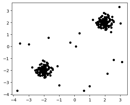

from sklearn.neighbors import LocalOutlierFactor
clf = LocalOutlierFactor(n_neighbors=20, contamination=0.1)
y_pred = clf.fit_predict(X) # 1: inlier, -1: outlier
outlier_mask = y_pred == -1

plt.figure(figsize=(5, 4))
plt.scatter(X[:, 0], X[:, 1], color='b', s=20, label='Inliers')
plt.scatter(X[outlier_mask, 0], X[outlier_mask, 1], color='r', s=50,label='Outliers')
plt.xlabel("Feature 1")
plt.ylabel("Feature 2")
plt.legend()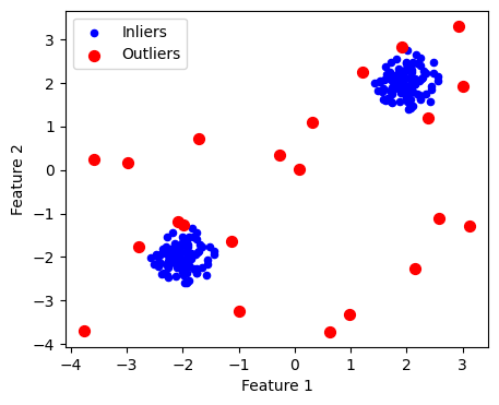

from sklearn.ensemble import IsolationForest
clf2 = IsolationForest(contamination=0.1)
# contamination : 이상치 비율
# n_estimators : 나무의 갯수 (defalut 100)
# max_features : 각 나무별 특성변수의 갯수(default 1)
clf2.fit( X )
y_pred2 = clf2.predict( X ) # 1: inlier, -1: outlier
outlier_mask2 = y_pred2 == -1

plt.figure(figsize=(5, 4))
plt.scatter(X[:, 0], X[:, 1], color='b', s=20, label='Inliers')
plt.scatter(X[outlier_mask2, 0], X[outlier_mask2, 1], color='r', s=50,label='Outliers')
plt.xlabel("Feature 1")
plt.ylabel("Feature 2")
plt.legend()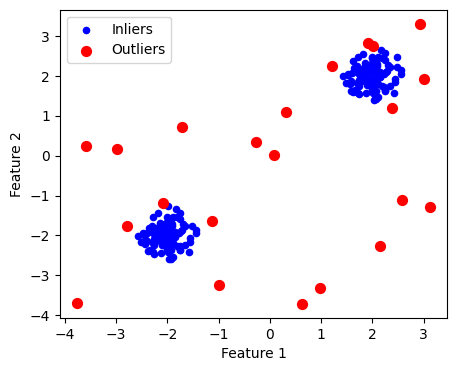

clf2.score_samples(X)

array([-0.39567479, -0.43973362, -0.38576701, -0.4625295 , -0.39169087,
       -0.39353101, -0.44632054, -0.4539587 , -0.39410011, -0.42823486,
       -0.43802322, -0.4231585 , -0.38600184, -0.40324911, -0.38778406,
       -0.46849881, -0.4075734 , -0.43420431, -0.45140279, -0.4113938 ,
       -0.40036102, -0.38335266, -0.42666089, -0.41104579, -0.44476313,
       -0.38744281, -0.39942914, -0.44257912, -0.38938554, -0.40470075,
       -0.39006555, -0.42881353, -0.44275864, -0.40154039, -0.39729665,
       -0.42434279, -0.42743206, -0.57699503, -0.38628797, -0.45454533,
       -0.3864026 , -0.44513991, -0.39598029, -0.41231495, -0.39270763,
       -0.40568073, -0.39005843, -0.43210962, -0.38601781, -0.38485125,
       -0.41991455, -0.40181793, -0.38788591, -0.48400217, -0.38538727,
       -0.47693547, -0.50815903, -0.39115267, -0.40423505, -0.43216634,
       -0.4254748 , -0.48475901, -0.4890737 , -0.40357175, -0.39439224,
       -0.42406868, -0.40171635, -0.44870204, -0.38761922, -0.43170548,
       -0.42364173, -0.43593615, -0.39560581, -0.4391784 , -0.39543452,
       -0.38550106, -0.38910014, -0.39558501, -0.48693408, -0.41865632,
       -0.40964165, -0.43730378, -0.41716448, -0.47893783, -0.39791987,
       -0.40492088, -0.38431516, -0.39544321, -0.42208103, -0.53522817,
       -0.41839783, -0.40171635, -0.39362168, -0.39333773, -0.44128807,
       -0.40208128, -0.40907841, -0.39096216, -0.38929625, -0.40645206,
       -0.38953796, -0.43147334, -0.38691831, -0.45292849, -0.39365031,
       -0.40064735, -0.46513506, -0.48209563, -0.39635657, -0.44569517,
       -0.4496465 , -0.43243444, -0.39406682, -0.40625773, -0.39826724,
       -0.46462545, -0.40782229, -0.42572527, -0.46599338, -0.42852596,
       -0.40082304, -0.38971614, -0.4628486 , -0.4219109 , -0.46365237,
       -0.39237271, -0.40320941, -0.42432754, -0.40309339, -0.40204058,
       -0.39044555, -0.43501511, -0.4324525 , -0.40503508, -0.40259674,
       -0.42956023, -0.42799201, -0.56257644, -0.38875652, -0.47585014,
       -0.3835507 , -0.4556408 , -0.406217  , -0.40385118, -0.39458774,
       -0.40122018, -0.40401747, -0.4443972 , -0.38320086, -0.3834212 ,
       -0.44945534, -0.4060406 , -0.38476589, -0.46817324, -0.38466101,
       -0.47610349, -0.49275615, -0.38344594, -0.40974845, -0.42395885,
       -0.42189161, -0.49261883, -0.48518689, -0.40901991, -0.39452123,
       -0.44785724, -0.40375287, -0.45749968, -0.40496115, -0.4260838 ,
       -0.41810669, -0.44560803, -0.38806155, -0.45523273, -0.38817405,
       -0.38177641, -0.39724261, -0.40279204, -0.46677259, -0.42162856,
       -0.4086809 , -0.43961327, -0.40404401, -0.45862325, -0.40473907,
       -0.41509113, -0.38081908, -0.39036169, -0.42441162, -0.52130968,
       -0.41557892, -0.40347146, -0.39318444, -0.38921027, -0.46342999,
       -0.39756969, -0.41357841, -0.38429305, -0.40297782, -0.40881293,
       -0.60259641, -0.44411547, -0.57052254, -0.50247903, -0.73212838,
       -0.64786135, -0.55623141, -0.45375541, -0.68754218, -0.67833274,
       -0.70698798, -0.63422967, -0.64031155, -0.78183101, -0.65477657,
       -0.67178443, -0.67084008, -0.68580391, -0.71446705, -0.64861428])