bank['marital'].value_counts()# 결혼 여부는 싱글/결혼/이혼 3진변수임. 순서가 없으므로 원-핫 인코딩으로 처리 예정
marital
married     2797
single      1196
divorced     528
Name: count, dtype: int64
bank['education'].value_counts()# 학력에 대한 내용은 primary - secondary - tertiary 순이므로 1~3 라벨인코딩 처리 예정# unknown은 학력수준이 낮을 가능성이 높을 것으로 추정, 0으로 처리하여 하나의 응답값으로 간주함.
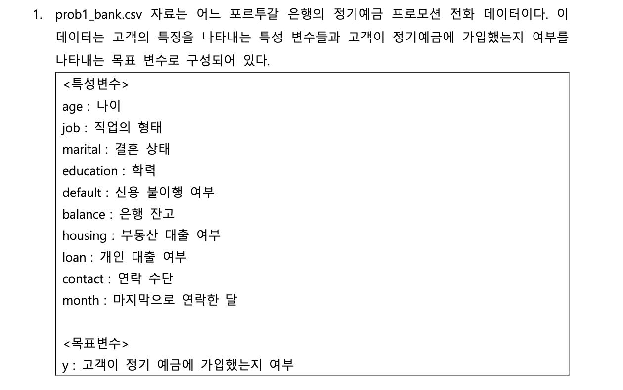
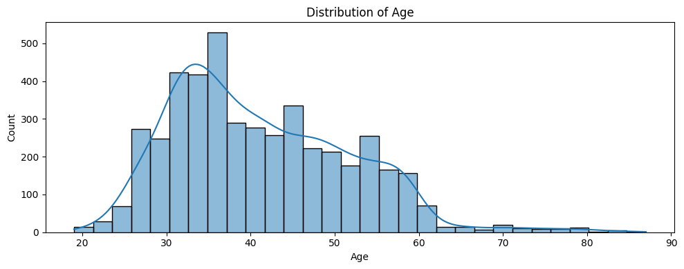
import matplotlib.pyplot as pltimport seaborn as sns# 1. age 분포plt.figure(figsize=(10, 4))sns.histplot(bank['age'], bins=30, kde=True)plt.title("Distribution of Age")plt.xlabel("Age")plt.ylabel("Count")plt.tight_layout()plt.show()# 2. balance 분포plt.figure(figsize=(10, 4))sns.histplot(bank['balance'], bins=30, kde=True)plt.title("Distribution of Balance")plt.xlabel("Balance")plt.ylabel("Count")plt.tight_layout()plt.show()
bank['age'].describe()# age는 오른쪽 skew가 미세하게 있는 정규분포와 가까운 형태. 표준화만 진행
count    4521.000000
mean       41.170095
std        10.576211
min        19.000000
25%        33.000000
50%        39.000000
75%        49.000000
max        87.000000
Name: age, dtype: float64
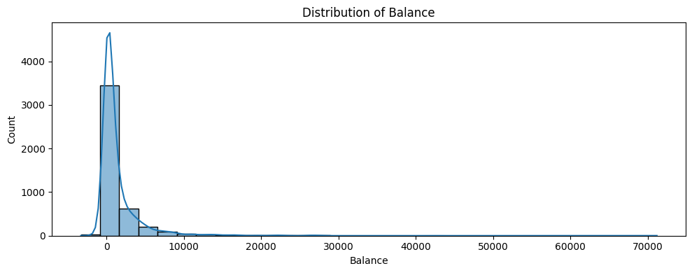
bank['balance'].describe()# balance는 음수도 존재하고, 값이 매우 극단적으로 치우쳐져 있는 형태. log변환 및 표준화 진행# 이후 LOF 방식으로 두 수치형변수에 대한 이상치 탐지, 약 1% 수준의 이상치 제거 예정
count     4521.000000
mean      1422.657819
std       3009.638142
min      -3313.000000
25%         69.000000
50%        444.000000
75%       1480.000000
max      71188.000000
Name: balance, dtype: float64
# 이상치 1%가 제거된 것을 확인할 수 있음bank_clean = bank[bank['is_outlier'] ==0].copy()bank_clean
age
education
default
balance
housing
loan
contact
month
y
job_blue-collar
...
job_student
job_technician
job_unemployed
job_unknown
marital_married
marital_single
log_balance
std_log_balance
std_age
is_outlier
0
30
1
0
1787
0
0
2
9
0
False
...
False
False
True
False
True
False
8.537388
0.431049
-1.056270
0
1
33
2
0
4789
1
1
2
4
0
False
...
False
False
False
False
True
False
9.000113
1.608188
-0.772583
0
2
35
3
0
1350
1
0
2
3
0
False
...
False
False
False
False
False
True
8.447843
0.203253
-0.583458
0
3
30
3
0
1476
1
1
0
5
0
False
...
False
False
False
False
True
False
8.474494
0.271052
-1.056270
0
4
59
2
0
0
1
0
0
4
0
True
...
False
False
False
False
True
False
8.106213
-0.665829
1.686036
0
...
...
...
...
...
...
...
...
...
...
...
...
...
...
...
...
...
...
...
...
...
...
4515
32
2
0
473
1
0
2
6
0
False
...
False
False
False
False
False
True
8.239593
-0.326519
-0.867145
0
4516
33
2
0
-333
1
0
2
6
0
False
...
False
False
False
False
True
False
8.000349
-0.935138
-0.772583
0
4518
57
2
0
295
0
0
2
7
0
False
...
False
True
False
False
True
False
8.191463
-0.448959
1.496912
0
4519
28
2
0
1137
0
0
2
1
0
True
...
False
False
False
False
True
False
8.401109
0.084364
-1.245394
0
4520
44
3
0
1136
1
1
2
3
0
False
...
False
False
False
False
False
True
8.400884
0.083793
0.267602
0
4475 rows × 26 columns
2.1.3 (3)
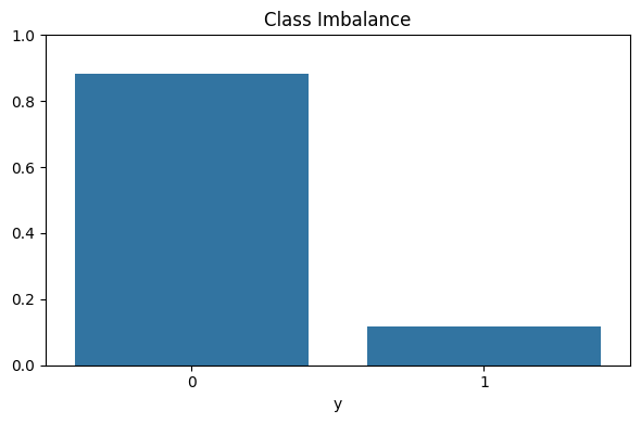
주어진 자료에 클래스 불균형이 있는지 확인한 뒤, 이에 대한 적절한 전처리 방법을 선택하여 진행하여라.
# 약 9:1로 0(No)의 비율이 압도적으로 많음. 클래스불균형 존재class_counts = bank_clean['y'].value_counts(normalize=True)plt.figure(figsize=(6, 4))sns.barplot(x=class_counts.index, y=class_counts.values, legend=False)plt.title("Class Imbalance")plt.xlabel("y")plt.ylim(0, 1)plt.tight_layout()plt.show()
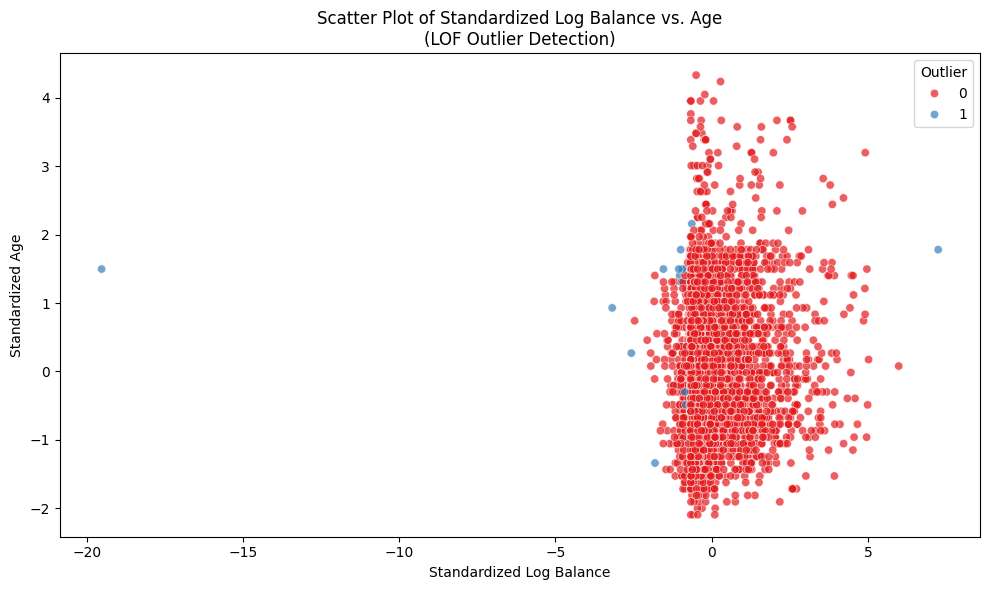
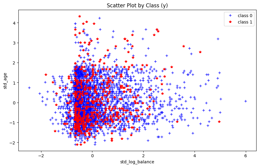
# 수치형 변수의 scatter plot상으로 특정 수치형 변수에 따른 치우침은 관측되지 않음.X = bank_clean[['std_log_balance','std_age']]y = bank_clean['y']plt.figure(figsize=(10, 6))plt.plot(X.loc[y ==0, 'std_log_balance'], X.loc[y ==0, 'std_age'], 'b+', label="class 0")plt.plot(X.loc[y ==1, 'std_log_balance'], X.loc[y ==1, 'std_age'], 'r*', label="class 1")plt.legend()plt.xlabel("std_log_balance")plt.ylabel("std_age")plt.title("Scatter Plot by Class (y)")plt.show()
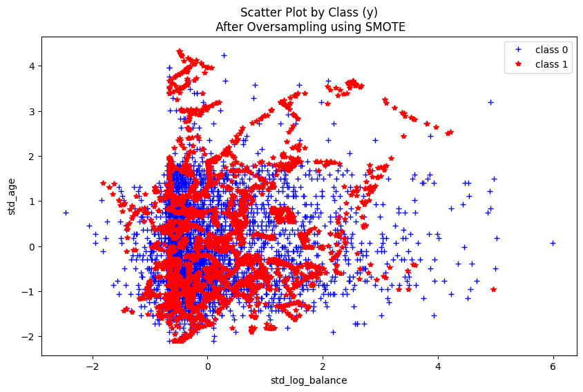
# 표본의 수가 적은 편이므로 oversampling 진행# 데이터의 구조가 그다지 복잡하지 않아 SMOTE 알고리즘을 적용하여 처리from imblearn.over_sampling import SMOTEoversample1 = SMOTE()OX, Oy = oversample1.fit_resample(X, y)plt.figure(figsize=(10, 6))plt.plot(OX.loc[Oy ==0, 'std_log_balance'], OX.loc[Oy ==0, 'std_age'], 'b+', label="class 0")plt.plot(OX.loc[Oy ==1, 'std_log_balance'], OX.loc[Oy ==1, 'std_age'], 'r*', label="class 1")plt.legend()plt.xlabel("std_log_balance")plt.ylabel("std_age")plt.title("Scatter Plot by Class (y)\n After Oversampling using SMOTE")plt.show()
from sklearn.cluster import KMeansfrom sklearn.metrics import silhouette_score# CUST_ID는 클러스터링에 사용하지 않으므로 제거X = df.drop(columns=["CUST_ID"])# 표준화scaler = StandardScaler()X_scaled = scaler.fit_transform(X)scaled_df = pd.DataFrame(X_scaled, columns=X.columns)# 최적 K 탐색inertia_list = []silhouette_list = []K_range =range(2, 11)for k in K_range: kmeans = KMeans(n_clusters=k, random_state=42, n_init=10) labels = kmeans.fit_predict(X_scaled) inertia_list.append(kmeans.inertia_) silhouette_list.append(silhouette_score(X_scaled, labels))best_k = K_range[silhouette_list.index(max(silhouette_list))]# K평균 군집화 결과 : 6개의 군집으로 분류되었으며, 갯수는 32개~3200개로 천차만별kmeans_final = KMeans(n_clusters=best_k, random_state=42, n_init=10)scaled_df["KMeans_Label"] = kmeans_final.fit_predict(X_scaled)summary_table_kmean = scaled_df.groupby("KMeans_Label").mean()summary_table_kmean["Count"] = scaled_df.groupby("KMeans_Label").size()summary_table_kmean
BALANCE
BALANCE_FREQUENCY
PURCHASES
PURCHASES_FREQUENCY
PURCHASES_TRX
Count
KMeans_Label
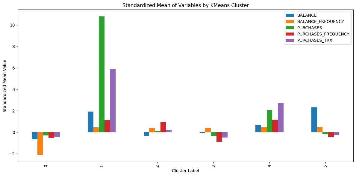
0
-0.679901
-2.105347
-0.305189
-0.528487
-0.414547
1390
1
1.906921
0.444930
10.782703
1.119309
5.892989
32
2
-0.331950
0.368356
0.087095
0.960328
0.227857
3253
3
-0.068576
0.366930
-0.369541
-0.895659
-0.502261
2989
4
0.696282
0.475045
2.042474
1.179006
2.713984
502
5
2.320551
0.483046
-0.159336
-0.433551
-0.273897
784
# K평균 군집화 시각화summary_table_kmean.drop(columns="Count").plot.bar(figsize=(12, 6))plt.title("Standardized Mean of Variables by KMeans Cluster")plt.xlabel("Cluster Label")plt.ylabel("Standardized Mean Value")plt.tight_layout()
2.2.2 (2)
주어진 자료에 DBSCAN Clustering 알고리즘을 적용하여, 적절한 군집을 생성하여라.
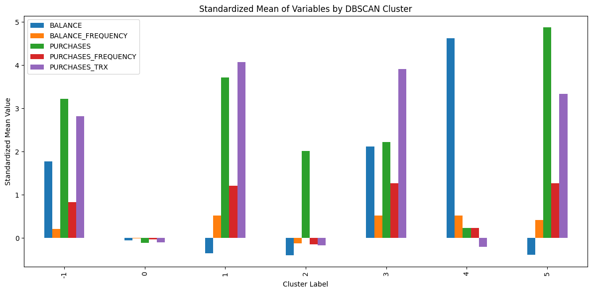
from sklearn.cluster import DBSCAN# DBSCAN 분류 : eps 및 min_samples는 여러번 반복을 통해 최적의 조합을 도출하였음.# 기준 : 분류가 너무 많거나 적지 않도록(3~6개), 너무 숫자가 적은 분류가 없도록dbscan = DBSCAN(eps=0.6, min_samples=4)labels = dbscan.fit_predict(X_scaled)# 라벨을 데이터프레임에 추가scaled_df["DBSCAN_Label"] = labels# DBSCAN 군집화 결과 : 잡음(-1)이 약 2% 포함되어있으며, 총 5개의 군집으로 분류(177개~6200개)summary_table_db = scaled_df.drop(columns="KMeans_Label").groupby("DBSCAN_Label").mean()summary_table_db["Count"] = scaled_df.groupby("DBSCAN_Label").size()summary_table_db
BALANCE
BALANCE_FREQUENCY
PURCHASES
PURCHASES_FREQUENCY
PURCHASES_TRX
Count
DBSCAN_Label
-1
1.776034
0.211613
3.221764
0.832535
2.823087
261
0
-0.056781
-0.007807
-0.107234
-0.028259
-0.094781
8657
1
-0.355658
0.518084
3.714917
1.207553
4.079060
10
2
-0.397981
-0.121515
2.012334
-0.148985
-0.169367
6
3
2.124764
0.518084
2.221881
1.269843
3.919140
8
4
4.623668
0.518084
0.235086
0.231676
-0.199541
4
5
-0.384296
0.422144
4.876114
1.269843
3.340815
4
summary_table_db.drop(columns="Count").plot.bar(figsize=(12, 6))plt.title("Standardized Mean of Variables by DBSCAN Cluster")plt.xlabel("Cluster Label")plt.ylabel("Standardized Mean Value")plt.tight_layout()
2.2.3 (3)
(1)과 (2)의 두 군집 분석 결과를 비교하고, 더 타당한 모델을 선택하여라.
K평균 vs DBSCAN 군집화 결과 비교
항목
K평균
DBSCAN
클러스터 수
6개
6개 (-1 포함)
클러스터 구성
최소 32, 최대 3253명
최소 4, 최대 8657
이상치 처리
없음
-1로 261명 처리
군집별 특성
분류기준 명확하
분류기준 모호, 대부분 하나로 분류
시각적 해석력
변수별 차이 뚜렷
구분 어려움
결론 : 이 데이터에서는 K평균이 더 타당한 군집화 방법
2.2.4 (4)
(3)에서 선택된 최종 모델로 생성한 군집들의 고객 특성을 분석하여라.
K평균 군집화 군집별 특성
0 : 낮은 자산, 낮은 구매액, 낮은 구매횟수 -> 하위 고객군 (약 17.5%)
1 : 높은 자산, 높은 구매액, 높은 구매횟수 -> 부유하고 이용량 많은 VIP 고객군 (약 0.5%)
2 : 평균이하 자산, 평균적인 구매액, 평균이상 구매횟수 -> 일반 고객군 중 상위 이용고객 (약 35%)
3 : 평균적인 자산, 평균이하 구매액, 평균이하 구매횟수 -> 일반 고객군 중 하위 이용고객 (약 33%)
4 : 평균적인 자산, 높은 구매액, 높은 구매횟수 -> 평균적이나 카드 사용량이 많은 우량 고객군 (약 5%)
5 : 높은 자산, 낮은 구매액, 낮은 구매횟수 -> 부유하나 카드를 이용하지 않는 잠재 고객군 (약 9%)
2.2.5 (5)
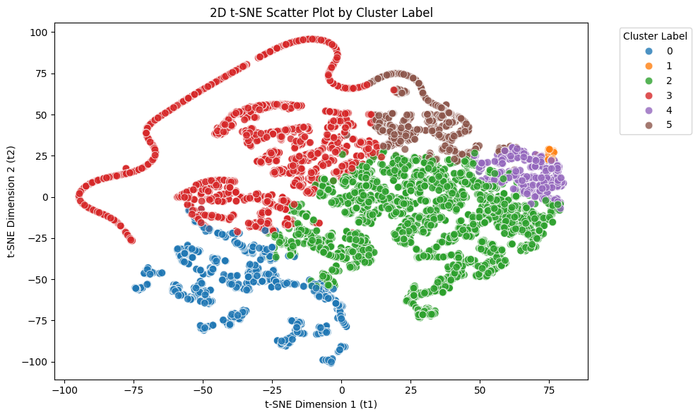
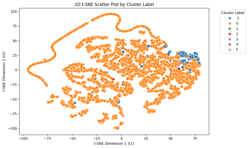
t-SNE 알고리즘을 적용하여 주어진 자료를 2차원으로 축소하여라. 그 결과를, (3)에서 선택한 모델의 군집 레이블에 따라 점의 색상이 다르게 표현된 2차원 산점도로 시각화하여라.
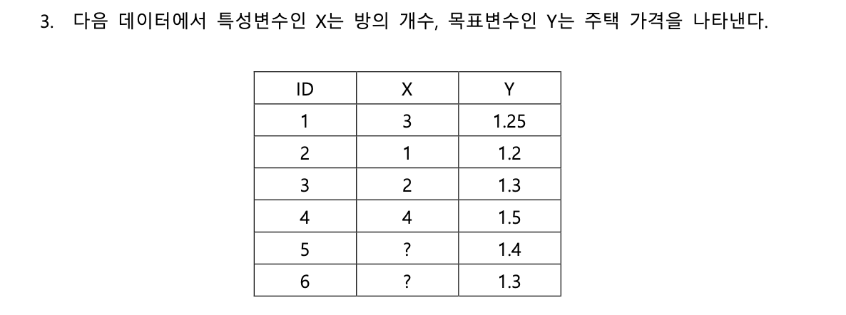
XGBoost 알고리즘을 적용하여 트리를 생성한다고 할 때, 첫번째 트리의 첫 마디에서 최적의 분리기준이 무엇인지를 구하여라. 단, 결측이 아닌 4개의 관찰치(ID 1~ID 4)만 이용할 것. 제곱오차 손실함수를 적용하며, 모델 초기값 𝑓0는 0.5로 두고, 규제 하이퍼 파라미터 𝜆는 0으로 설정할 것. 또한 계산 과정을 상세하게 서술할 것.